Model Training

This notebook exemplifies the Sierra Snow Model (SSM) (a derivation of the National Snow Model (NSM)) data processing (through the DataProcess.py script), and model training, predictions, and preliminary evaluation via the MLP_model.py script. With the focus of GeoSMART Hack Week to advance machine learning modeling skill sets, the motivation of the SSM project is for participants to modify the MLP_model.py script. Suggested modifications include optimizing the current multilayered-perceptron (MLP) neural network algorithm or selecting and optimizing a different ML algorithm (strongly encouraged). We encourage advanced modelers to contact Dr. Ryan Johnson (rjohnson18@ua.edu) for ideas and methods to optimize the model framework, there are several concepts of interest including feature engineering, domain optimization, feature selection, etc.

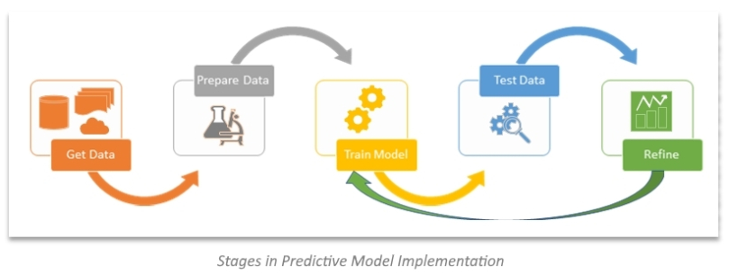
The following workflow exemplifies the steps and python files to process the training data, train a model, produce predictions, and perform preliminary evaluations

%pip install myst-nb pandas==1.4.3 rioxarray xarray contextily h5py tqdm tables scikit-learn seaborn tensorflow progressbar hydroeval  nbformat==5.7.0   matplotlib basemap numpy rasterio geopandas==0.10.2

import os
import DataProcess
#pip install h5py, tables, scikit-learn, seaborn, tensorflow, change pandas to 1.4.3 - %magic lines
import MLP_Model
import warnings; warnings.filterwarnings("ignore")
#Set working directories
#cwd = os.getcwd()
#os.chdir("..")
#os.chdir("..")
#datapath = os.getcwd()  
#cwd = '/home/jovyan/shared/geosmart-hackweek-2023/snow-extrapolation/Predictions/'
datapath ='/home/jovyan/shared-public/snow-extrapolation-web/'

Model Training and Testing Schema

The motivation the project is to advance the SSM skill for extrapolating regional SWE dynamics from in-situ observations. To develop and test the SSM, we will train the model on NASA Airborne Snow Observatory (ASO) and snow course observations spanning 2013-2018, and some of 2019. Within this training dataset, model training will use a random 75-25% train-test data split. The random sample function will be 1234 to ensure all participants models use the same training and testing data for this phase of model development - note, this will support an intermodel comparision.

Model validation will be on water year 2019 and use the SSM_2019_Simulation. This historical simulation will function as a hindcast, and use the 2019 water year NASA ASO and snow course observations to determine model performance.

Upon the completion of model training, model execution predicts 1-km resolution SWE from data up to the current date of observation provided Latitude, Longitude, corresponding topographic data, and neighboring observation input features. From the sampling of test features, Chapter evaluation notebook compares the modeled 1-km grid SWE values to the observed values.

#Define hold out year -need Shard Model folder  
HOY = 2019
#Run data processing script to partition key regional dataframes
#note, need to load RegionTrain_SCA.h5,
RegionTrain, RegionTest, RegionObs_Train, RegionObs_Test, RegionTest_notScaled = DataProcess.DataProcess(HOY, datapath, datapath)

Multilayered Precepton Network (MLP)

Given the identified optimal feature sets using recursive feature elimination (RFE), this step trains your model. Here, the model is an ANN multilayer perceptron (MLP) regression model to estimate SWE found in the MLP_Model file. This file serves as a template for Hackweek participants to modify and by following the template, participants will be able to streamline model development and evaluation.

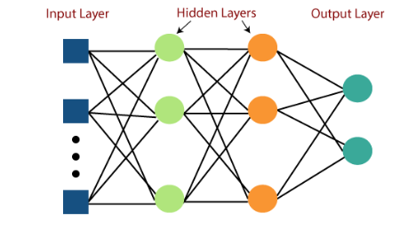
The MLP is a classical type of feedforward ANN, successfully and frequently applied in environmental modeling applications. The MLP regression model estimates a target variable by learning a non-linear function to describe the target from an input vector of features. It performs learning via a back-propagation algorithm over a series of hidden layers containing interconnected nodes (neurons). The neurons connect bordering layers by a summation of weights and an activation function transforms model outputs to predicted values (i.e., SWE (in)). The model calculates error and adjusts the weights to minimize the error during model training, supporting the use of MLPs to effectively describe a target variable with any function, continuous or discontinuous.

Model training leveraged the Keras API within the TensorFlow library. We selected the popular, open-source TensorFlow and Keras platforms for their wide applicability and capabilities in deep learning. The MLP model for the region consists of an input layer containing nodes for each feature in the optimized feature space, 7 dense hidden layers, and an output layer of the target SWE value. Model formulation uses the Rectified Linear Unit (ReLu) activation function to transform each hidden layer to non-linearize the solution.

#model training, each participants model will be different but should follow the prescribed input feature template
epochs= 60
MLP_Model.Model_train(datapath, epochs, RegionTrain, RegionTest, RegionObs_Train, RegionObs_Test)

Make predictions on the random sample of testing data

The next phase of model development is to examine model performance on the random sample of testing data. Refining model predictions at this phase will ensure the best model performance for the Hold-Out-Year validation set.

#Need to create Predictions folder if running for the first time
Predictions = MLP_Model.Model_predict(datapath,  RegionTest, RegionObs_Test, RegionTest_notScaled)

Perform Preliminary Model Evaluation

How does your model performance? We are using simple model evaluation metrics of R2 and RMSE to guage model performance. You will perform a more exhaustive model evaluation in the Evaluation chapter.

Performance = MLP_Model.Prelim_Eval(datapath, Predictions)
Performance

Model Evaluation

Now that we have a trained model producing acceptable performance, it is time to more rigorously evaluate its performance within an interactive evaluation notebook.